Damping

When an external force acts on an oscillating system, it can gradually cause the system to lose energy. This energy loss leads to a decrease in amplitude over time, ultimately creating a state of equilibrium. Damping refers to reducing or dissipating the energy of oscillations or vibrations in a system. The energy is dissipated usually in the form of heat, which leads to a gradual reduction in the motion of the oscillating system.

Examples of damping include:

Shock absorbers in vehicles
Seismic dampers in buildings
Vibration dampers on bridges

Types of Damping

Depending on the system’s nature, damping can occur through various mechanisms, such as frictional forces, air resistance, or electrical resistance.

1. Viscous Damping

Viscose damping is caused by fluid resistance and occurs when bodies move at moderate speeds through fluid mediums such as air, gas, water, or oil. This is the most commonly used damping mechanism to reduce the amplitude of vibrations. In this type of damping, the resisting force is proportional to the relative velocity of the vibrating body.

2. Coulomb Damping

This type of damping occurs due to the friction between sliding dry surfaces. The friction force remains nearly constant and depends on the characteristics of the sliding surfaces and the normal pressure between them.

3. Structural Damping

The damping arises from the friction between internal planes that slip or slide as the material deforms. It is also known as hysteresis damping. For a vibrating body, the stress-strain diagram is not a straight line but forms a hysteresis loop, the area of which represents the energy dissipated to molecular friction per cycle per unit volume.

4. Magnetic Damping

This damping is observed when vibrating, oscillating, or rotating conductors in a magnetic field gradually return to rest. It is caused by eddy currents generated by the system’s movement within the magnetic field.

Damping Equation

The damping equation provides a mathematical representation of the damping force acting on a system. This force opposes the motion and helps dissipate energy, reducing the amplitude as time progresses. The damping equation in one dimension is commonly described by the following second-order ordinary differential equation (ODE):

\[ m \frac{d^2x}{dt^2} + c \frac{dx}{dt} + kx = 0 \]

Where:

– m is the mass of the system

– c is the damping coefficient

– k is the spring constant

– x is the displacement of the system from its equilibrium position

– t is time

For a system consisting of a harmonic oscillator, this equation is called the damped harmonic oscillator equation.

Important Parameters

1. Damping Coefficient (c): It quantifies the amount of resistance or frictional force opposing the system’s motion. This resistance leads to the dissipation of energy, causing the amplitude of oscillations to decrease over time.

2. Damping Force (F_d): The force responsible for damping. It is proportional to the velocity and opposite to the direction of motion.

\[ F_d = – c\frac{dx}{dt} \]

3. Undamped Natural Frequency (ω_o): The frequency at which the system oscillates when no damping is present. It is a fundamental system property and depends only on the system’s mass and spring constant.

\[ \omega_o = \sqrt{\frac{k}{m}} \]

4. Damped Natural Frequency (ω_d): The frequency at which the system oscillates when damping is introduced. Aside from mass and spring constant, it depends on the damping coefficient.

\[ \omega_d = \sqrt{\omega_o^2 – \left( \frac{c}{2m}\right) ^2} \]

5. Damping Ratio (ζ): It is a dimensionless quantity to measure damping and describes how oscillations in a system decay after a disturbance.

\[ \zeta = \frac{c}{2\sqrt{mk}} \]

Damping Resonance

When a system is driven by an external periodic force, its response can be significantly affected by the interplay between the driving frequency and its natural frequency, as well as the presence of damping. Resonance occurs when the frequency of the external force (driving frequency) is close to the system’s damped natural frequency. At resonance, even a small periodic force can produce large amplitude oscillations because the system absorbs energy efficiently from the external source.

Example: A group of soldiers is marching in unison across a suspension bridge. The rhythmic footsteps of the soldiers match the natural frequency of the bridge, leading to resonance.

The damped resonance behavior can be described mathematically by the following equation:

\[ m \frac{d^2x}{dt^2} + c \frac{dx}{dt} + kx = F_o \cos(\omega t) \]

Where:

– m is the mass

– c is the damping coefficient

– k is the spring constant

– F_o is the amplitude of the external force

– ω is the frequency of the external force or driving frequency

– x is the displacement from the equilibrium

For a system consisting of a harmonic oscillator, this equation is called the driven harmonic oscillator equation.

The difference between the damped and the driven harmonic oscillator equations is that in the former, the right-hand side is zero, while in the latter, it consists of the sinusoidal driving force. As a result, there is no resonance in the damped harmonic oscillator in the traditional sense. The system’s response depends on the initial conditions and the damping factor, which we will explore in the next section.

Damping Equation Solutions

The solutions to the damping equation reveal critical information about the system’s behavior over time. It tells us how quickly oscillations decay, the rate at which energy is dissipated, and the nature of the system’s return to equilibrium.

In the case of damping resonance, solving the driven harmonic oscillator equation reveals how the displacement varies with time under the influence of the external force. The solutions indicate how the system’s amplitude and phase change with different driving frequencies and damping levels. The response is influenced by the damping ratio ζ and exhibits different behaviors based on its value.

By solving the damping equation, we can classify the system’s response as underdamped, critically damped, or overdamped, each with distinct characteristics.

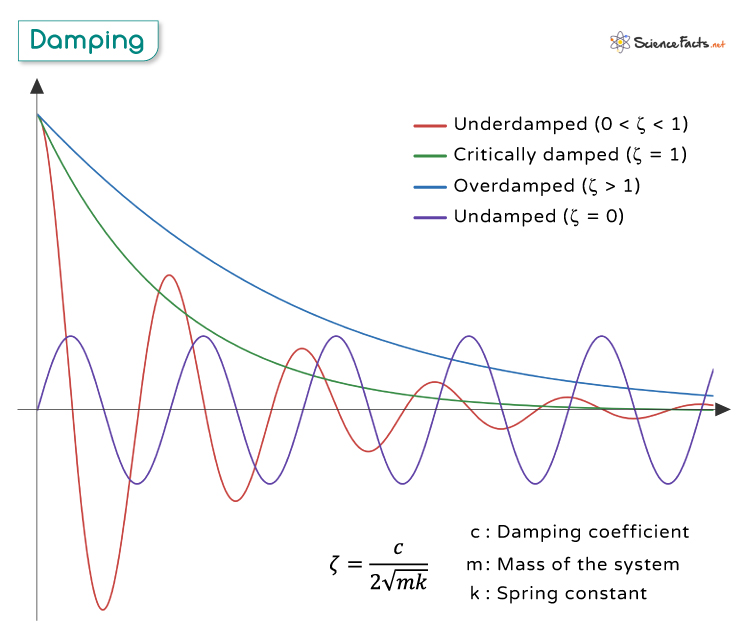
1. Underdamped

The system is said to be underdamped when c² < 4mk or 0 < ζ< 1. The solution takes the form:

\[ x(t) = e^{-\frac{c}{2m}t} \{A \cos\left(\omega_d t\right) + B \sin\left(\omega_d t\right)\} \]

Where A and B are constants determined by the system’s initial conditions.

The system shows oscillatory behavior with a decreasing amplitude over time due to damping.

Resonance Condition for Driven Harmonic Oscillator

Resonance occurs when the driving frequency ω is close to the damped natural frequency ω_d. The displacement response is maximized, and the system oscillates at the resonance frequency given by

\[ \omega_r = \sqrt{\omega_o^2 – \left( \frac{c}{2m}\right) ^2} \]

2. Critically Damped

The condition for critically damped is c² = 4mk or ζ = 1. The solution is given by:

\[ x(t) = (A + Bt) e^{-\frac{c}{2m}t} \]

Where A and B are constants determined by the system’s initial conditions.

The system returns to equilibrium as quickly as possible without oscillating. It does not exhibit resonance because the driving force cannot induce oscillations at a specific frequency to achieve maximum amplitude, and the system’s response decreases monotonically as the driving frequency increases.

3. Overdamped

The system is said to be overdamped when c² > 4mk or ζ > 1. The solution leads to a non-oscillatory behavior given by:

\[ x(t) = C_1 e^{r_1t} + C_2e^{r_2t} \]

Where:

r₁ and r₂ are the roots of the characteristic equation: mr² + cr + k = 0
C₁ and C₂ are constants determined by the system’s initial conditions.

Like the critically damped case, the system does not exhibit a traditional resonance peak because the damping is too strong to allow significant oscillations. The amplitude decreases monotonically with increasing driving frequency.

Example Problem

A mass-spring system has a mass (m) of 2 kg, a damping coefficient (c) of 8 Ns/m, and a spring constant (k) of 50 N/m. The system is subjected to an external force F(t) = 10 cos(2t) N. Determine the response of the system for t ≥ 0.

Solution:

The equation of motion for the damped harmonic oscillator is given by:

\[ m \frac{d^2x}{dt^2} + c \frac{dx}{dt} + kx = F(t) \]

Substituting the given values, we get:

\[ 2 \frac{d^2x}{dt^2} + 8 \frac{dx}{dt} + 50x = 10 \cos(2t) \]

It is a non-homogeneous second-order linear differential equation. To solve it, we first find the characteristic equation by setting the homogeneous part equal to zero:

\[ 2r^2 + 8r + 50 = 0 \]

Solving this quadratic equation, we find two complex roots:

\[ r = -2 + \sqrt{21} i \quad \text{and} \quad r = -2 – \sqrt{21}i \]

The general solution for the homogeneous part is then:

\[ x(t) = e^{−2t}\{A \cos(\sqrt{21}t)+B \sin (\sqrt{21}t)\} \]

Now, we need to find a particular solution for the non-homogeneous part. Since the external force is a cosine function, we assume a particular solution of the form:

\[ x_p(t) = C \cos(2t) + D \sin(2t) \]

Substituting x_p(t) and x_h(t) into the non-homogeneous differential equation and equating coefficients gives us the values of C and D, and the particular solution becomes:

\[ x_p(t) = 0.208 \cos(2t) + 0.079 \sin(2t) \]

After finding x_p(t), the general solution for the entire system is given by the sum of the homogeneous and particular solutions:

\[ x(t) = x_h(t) + x_p(t) \]

\[ \text{Or,}\hspace{0.3 cm} x(t) = e^{−2t}\{A \cos(\sqrt{21}t)+B \sin (\sqrt{21}t)\} + 0.208 \cos(2t) + 0.079 \sin(2t) \]

Thus, the above equation fully describes the system’s response over time. The initial conditions, which are not provided in the problem statement, determine the constants A and B.