Acceleration
Suppose an object moves from one point to another such that its velocity at the initial point is different from that at the final point. Acceleration is defined as the rate at which the velocity changes. It is a vector quantity having both magnitude and direction.
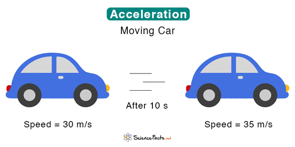
To understand acceleration, let us take a numerical example. An object starts from rest and picks up speed such that its velocity becomes 5 m/s in 10 seconds. It took 10 s to go from 0 m/s to 5 m/s. Then, the rate at which its velocity changed is: (5 m/s – 0)/10 s = 0.5 m/s2. Therefore, its acceleration is 0.5 m/s2.
Examples
- A plane taking off
- Pressing the gas pedal of a car
- A roller coaster riding on its tracks
- A fruit falling from a tree
- Throwing a football
- Going up and down an elevator
Equation
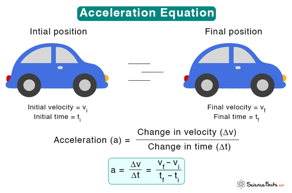
Average Acceleration
Acceleration is the rate of change of velocity. In other words, it is the change in velocity over a given time interval. Suppose vi and vf are the initial and final velocities of the object at time ti and tf, respectively. Then, the average acceleration is
Where
Δv: Change in velocity
Δt: Time interval over which the change occurred
SI Unit: meters per second squared or m/s2
Imperial unit: feet per second squared or ft/s
Note:
- Acceleration and velocity must not be confused. Velocity is the change in position with respect to time. If the object moves with a constant velocity, then Δv = 0, and its acceleration is zero.
- In the above equation, acceleration is the change in velocity over the change in time. It does not mean that if the velocity is high, the acceleration is high, or if the velocity is low, the acceleration is low. The velocity can be high, the acceleration can still be low, and vice versa.
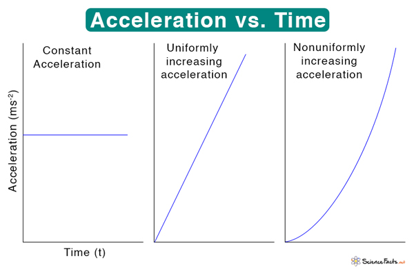
- If the velocity changes by equal amounts in equal time intervals, the acceleration will remain constant. It is known as uniform or constant acceleration. The graphs below illustrate the difference between constant acceleration, uniformly increasing acceleration, and nonuniformly increasing acceleration.
- Can acceleration be negative. Generally, acceleration refers to situations where the velocity increases with time. In this case, the acceleration is a positive quantity. However, if the velocity decreases with time, the magnitude of acceleration will be negative. The object slows down, and the phenomenon is called deceleration or retardation.
Instantaneous Acceleration
The average acceleration is measured over a long interval of time. On the other hand, instantaneous acceleration is the acceleration calculated for an infinitesimally small time interval. It can be found by setting the limit of the time interval in the above equation to zero.
Therefore, acceleration is the first derivative of the velocity with respect to time. Note that the velocity is the derivative of distance (x) over time. We can rewrite the above equation as
Therefore, acceleration is the second derivative of distance with respect to time.
Acceleration from Newton’s Second Law
Acceleration can also be calculated directly from Newton’s Second Law. According to this law, the net force (F) on an object is given by the product of its mass (m) and acceleration (a). Mathematically, it is represented by
Rearranging this equation gives the acceleration a.
Direction of Acceleration
The direction of acceleration depends on whether the object is speeding or slowing down and the direction of travel. Imagine a car traveling on a straight road such that it is speeding up. Its velocity increases with time. Its direction is along the direction of travel. Now, suppose the car is slowing down. Its velocity decreases with time. Its direction is opposite to the direction of travel. This type of acceleration, in which the acceleration vector is along the displacement vector, is called linear acceleration.
Suppose the car makes a turn around a curve path. Its velocity vector will change. We can use the concept of vector resolution to study its acceleration. Its velocity vector can be resolved into two components. One component is directed toward the center of curvature of the curve path, called the radial velocity. Another component is perpendicular to the radial velocity, called the tangential velocity. The rate of change of radial velocity is called radial acceleration and is directed radially inward. The rate of change of tangential velocity is called tangential acceleration. It is directed tangentially to the point under consideration on the curve path, as shown in the image below.
Suppose the car moves around a circular path. In that case, its radial acceleration is called centripetal acceleration, discussed in our article on centrifugal force.

Example Problems
Problem 1: A motorcyclist starts from rest and speeds up uniformly to 60 miles per hour (mph) in 12 seconds. What was the magnitude of the average acceleration of the motorcyclist?
Solution:
Given vi = 0, vf = 60 mph, Δt = 12 s
Let us convert mph to m/s.
60 mph = (60 miles x 1.6 km/mile x 1000 m/km)/(1 hr x 3600 s/hr) = 26.67 m/s
The acceleration is
a = (vf – vi)/Δt = (26.67 m/s – 0)/12 s = 2.22 m/s
Problem 2: A racehorse coming out of the gate accelerates from rest to a velocity of 14.0 m/s due in 1.90 s. What is its average acceleration?
Solution:
Given vi = 0, vf = 14 m/s, Δt = 1.9 s
The acceleration is
a = (vf – vi)/Δt = (14 m/s – 0)/1.9 s = 7.37 m/s
-
References
Article was last reviewed on Monday, January 2, 2023
Related articles


Join our Newsletter
Fill your E-mail Address